本文建议使用白色背景观看。
SAC
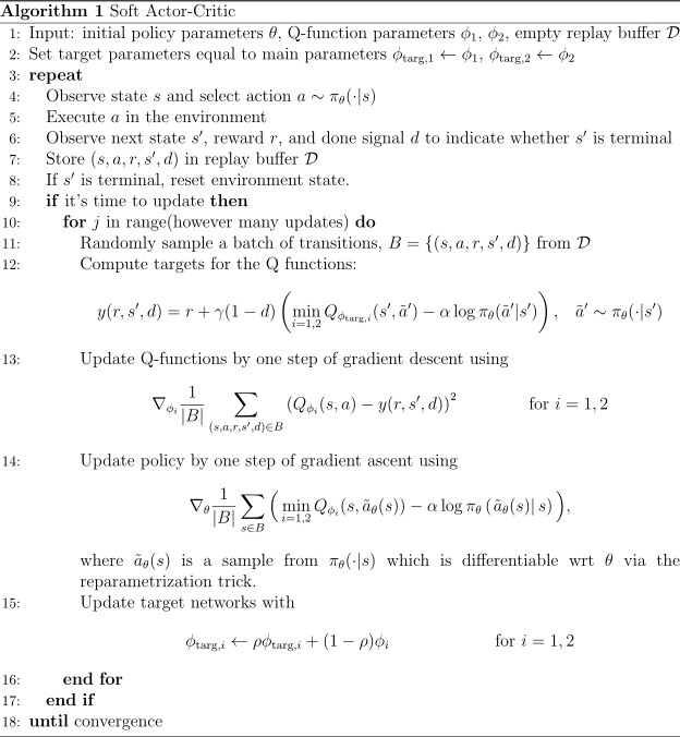
SAC: Soft Actor Critic,结合了DDPG的双Q函数降低over estimation bias, 以off-policy的方式,将最大熵加入到策略学习和Q函数学习的目标中,打破了传统的只看reward的唯一目标方式。数据存储在replay buffer中,使用经验回放的方式进行训练。SAC的目标是最大化期望奖励和策略熵的加权和:
$$ \pi^* = \arg \max_{\pi} \mathbb{E} \left[ \sum_{t=0}^\infty \gamma^t \left( R(s_t, a_t, s_{t+1}) + \alpha H(\pi(\cdot | s_t)) \right) \right] $$
其中, $$ [ H(P) = \underset{x \sim P}{\mathbb{E}} [-\log P(x)] ] $$
所以动作价值函数就变为:
$$ Q^{\pi}(s, a) = \mathbb{E} _{\tau \sim \pi} [ \sum _{t=0}^{\infty} \gamma^t R(s_t, a_t, s _{t+1}) + \alpha \sum _{t=1}^{\infty} \gamma^t H(\pi(\cdot|s_t)) \bigg| s_0 = s, a_0 = a] $$
Actor
输出的是动作的分布,网络建模了状态$s$到动作的均值和方差:$\mu,\sigma = f(s)$ 这里值得思考的是,actor网络建模状态到动作的不确定度,而不是像DDPG和TD3那样,固定一个动作的不确定度去做探索。这里的思路是:面对不同的环境状态,动作的输出不确定度是不同的:例如,想象一个场景,机械手抓取一个物体:在抓取的过程中,观察到的状态从视觉图像当中获取到被抓取物体的像素或者3D信息,在这个阶段,需要策略输出较确定的动作,从宏观看就是稳定地保持机械臂的位姿,手指的开口度也在缓慢的朝一个方向变化;当抓取到物体之后,我们对于机械手的位姿没有那么高的要求,所以在移动的过程中,就不需要太确定的动作,而这个过程视觉看到的像素也很有可能训练的时候没见过,那这时候,输出一个高方差的动作也不太影响成功率。如果固定方差,就会出现不同任务机械臂具有统一的动作不确定度,导致精细操作失败,大范围移动畏畏缩缩。 还要注意的是,在SAC中,需要对输出的动作做上下限处理,保证在动作空间内。actor网络的最后一层,是tanh激活函数,输出动作的均值$\mu$在[-1,1]之间。对于方差$\sigma$,SAC使用了一个技巧,网络输出的是log方差$\log\sigma^2$,然后通过指数函数得到方差$\sigma^2$,这样可以保证方差是正数。 actor网络的损失函数: $$ \begin{align*} \max _{\theta} \underset{\substack{s\sim\mathcal{D}\ \xi\sim\mathcal{N}}}{\mathbb{E}} \left[ \min _{j=1,2} Q _{\phi_j}(s,\tilde{a} _{\theta}(s,\xi)) - \alpha \log \pi _{\theta}(\tilde{a} _{\theta}(s,\xi)|s) \right] \end{align*} $$ 跟DDPG和TD3不同,第一项是从两个Q网络中找出较小的那个,然后加上熵。
Double Q Critic
价值优化的目标函数:
$$ L(\phi_i, \mathcal{D}) = \underset{(s,a,r,s’,d) \sim \mathcal{D}}{\mathbb{E}} \left[ \left( Q_{\phi_i}(s,a) - y(r,s’,d) \right)^2 \right] $$
其中,
$$ y(r, s’, d) = r + \gamma(1 - d) \left( \min_{j=1,2} Q_{\phi_{\text{tar}, j}}(s’, \tilde{a}’) - \alpha \log \pi_{\theta}(\tilde{a}’|s’) \right), \quad \tilde{a}’ \sim \pi_{\theta}(\cdot|s’). $$
与DDPG和TD3不同的是,用来做next-state-action价值评估的$a’$来源于actor网络,且该动作的不确定度也来源于actor网络,而不是target actor网络;target Q也加入了熵。
SAC整体的算法流程:
小结
SAC整体感觉是PPO和DDPG的结合体,既利用了off-policy的经验回放,又利用了最大熵的思想,解决了DDPG和TD3在高维动作空间下的探索问题。SAC的actor网络输出的是动作的分布,而不是固定的动作,但是又不像PPO,拿着动作概率去做重要性采样去梯度优化,而是间接通过Q函数,反过来判断什么样的状态可以输出大波动的动作,什么样的状态必须稳住,输出高稳定度的动作,训练阶段提供了探索性(动作分布一定会偏差于所需要的)。SAC的critic网络采用了Double Q结构,降低了overestimation bias。带来的好处:
- 在高维动作空间下,SAC的探索效率更高,能够更快地收敛到最优策略。
- 数据利用率高
- 想要提升Q估计的稳定性,对critic网络进行修改,具有很高的天花板
- 利用失败数据,类似于HER(Hindsight Experience Replay)系列工作,从失败中也能学到有价值的状态-动作对。
下面就开始看看基于SAC,近一两年出现了什么改进工作。
FlashSAC
FlashSAC基于SAC,属于off-policy。传统的强化学习网络设计2~3层,且主要是全连接,没有设计出深度更深的网络结构是因为反向传播有梯度丢失问题。 核心创新是扩大网络的规模,且设计网络结构去解决网络规模变大了之后的Q方差太大问题。
- 扩大数据规模,每次训练的参与数据变多,但是更新策略的频率变慢
- 稳定训练过程,限制Q网络的动态更新步幅
- 更广泛的动作探索空间
更高效的训练
大样本、小频率更新优于小样本、高频率更新
- 大规模并行仿真,获取数据:1024个环境同步交互采集数据。优势是对于高维度的动作空间,足够的数据覆盖是训练成功的关键
- 10M的replay buffer大小。
- 传统的RL神经网络是2-3层的MLP(0.2M~0.5M参数量),FlashSAC使用网络2.5M参数量,actor和critic都是6层,2048的batch size。1024个transition 更新2次网络参数,网络对数据的更新率低
更稳定的训练过程
这部分取决于网络结构的创新:
首先需要先写下OOD(Out-of_Distribution) 数据对于训练RL网络有什么样的影响。
来源:传感器数据噪声,或者是一个发生概率很小的事件对应的数据,尽管没有噪声,但是几乎不可能发生。
在训练的过程中,一个OOD数据,离群幅度很远,基于SAC考虑,如果当前的网络是target Q, 该网络是用来输出$y$的,那么,本次输出的target就会变得很夸张,反过来训练Q网络,就会拉偏参数,强行让参数去适应那个离谱的target,下一次来了正常数据,估计出来的Q也距离真实值很远,然后就会使得网络崩溃。这个问题的根源是RL本质是自举(Boostrap)的系统,要保证每一步的学习都是客观的,不能学偏。具体就是如果没有RMSNorm的话,经过激活函数之后,如果拿来做反向传播,原本好的网络参数会被这个OOD数据强行拉偏很多,如果网络是critic的话,就意味着对动作价值的估计产生很大的偏见,如果网络是actor的话,就会带歪最优策略,训练崩溃。
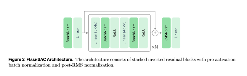
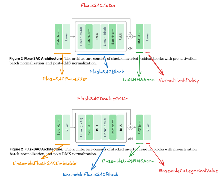
下面是FlashSAC的网络结构。actor和critic都采用了这种骨架,但是最精彩的是在critic部分,它参考了Addressing Function Approximation Error in Actor-Critic Methods,重点是稳定target Q,类似于SAC,TD3,都采用了两个target Q(或者更多,取决于参数num_qs),从replay buffer里面采样的Batch都会并行地通过每一个下图中的网络。在FlashSAC定义出来的每一个子网络结构中,采用了这篇论文的思想,着重解决Overestimation的问题。
网络结构的创新
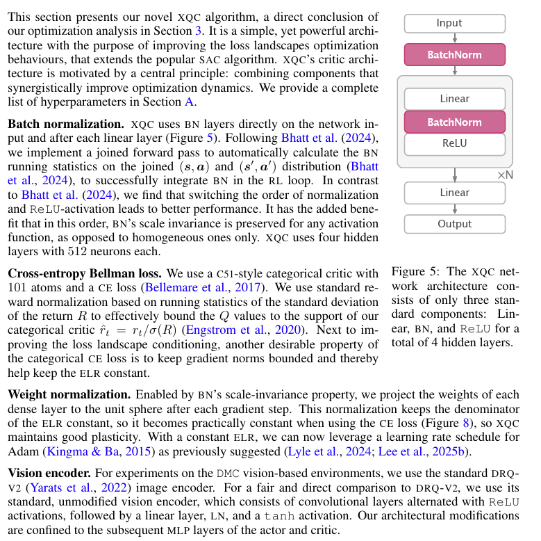
- 加入BN(BatchNormalization)
- 引入类似于Transformer feedforward子网络,在残差(residual)部分,本质上是一种专门为强化学习训练设计的深度神经网络骨架。它借鉴了计算机视觉领域的经典设计,核心思想是:先扩维,后降维,让网络能以更大的容量和更深的层数稳定运行。
- critic输出带分布的Q函数,利用这个分布调节奖励。
在强化学习中,replay buffer里面的数据,是由不断净化的actor和环境交互产生的,所以通过随机采样replay buffer的数据,分布就不属于一个策略,而是混合了很多历史策略的。这样的数据作为Batch输入到critic,直接通过线性层+ReLU,就会出现网络输出有巨大的抖动和尖峰,往往与实际情况不相符。Q有巨大的尖峰和抖动,造成Loss也会产生尖峰,在反向传播优化网络参数的时候,带偏参数。经过对数据的BN,相当于根据数据创建了本次采集的一个分布,且这个分布所代表的可能是多峰的,很好地刻画了数据,降低了输入的幅值差异,还不破坏后续训练所需要的输入信息。
数据侧混合了当前和下一时刻
和SAC相比, 参考了CrossQ:critic 网络接收到的状态输入是当前状态和下一状态的组合:$s_{t}+s_{t+1}$,接受到的动作输入是当前动作$a_{t}$和根据actor网络$\pi_{\theta}$,$a_{t+1}=\pi_{\theta}(s_{t+1})$采样出来的$a_{t+1}$。这样做的好处是因为网络的第一层就是BatchNorm,会将状态分布和动作分布做统一,利用这个统一了的分布,去预测target Q,这样能够保持预测的一致性和连续性。这部分也是最大化Q值估计稳定性的重要手段。
Cross-Batch Value Prediction. Batch normalization computes statistics per batch, so the predicted Q-values and target Q-values receive different normalization when computed in separate forward passes. Following [8], we concatenate current and next-state transitions into a single batch so that both share the same statistics, ensuring consistency in the Bellman update.
下面的代码得到了确认。
| |
Q网络输出除了价值,还有概率
本文参考了下文的网络结构重复的部分,但是没有用到LERP。
Hyperspherical Normalization for Scalable Deep Reinforcement Learning
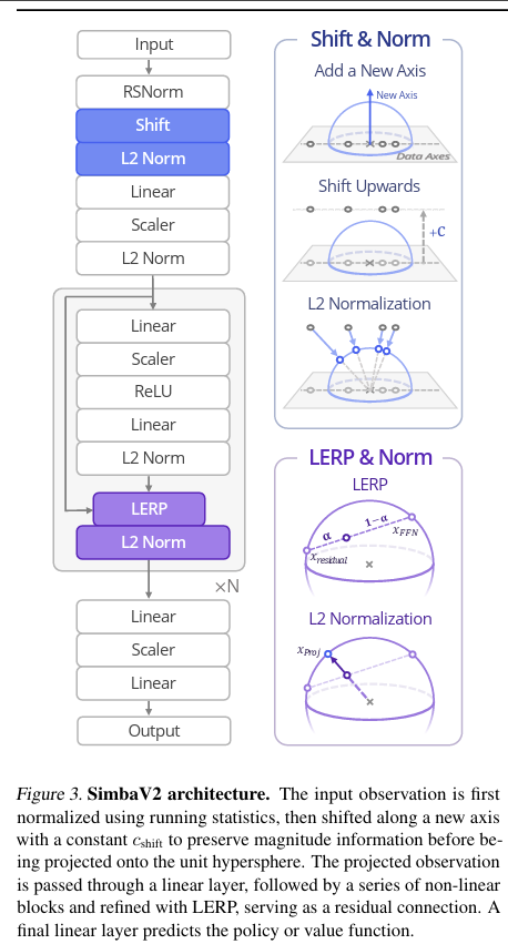 这篇文章引入了黎曼流形(Riemannian Optimization)的优化。
欧几里得空间的SGD的思路如下公式,通过输入的数据$\mathcal D$和监督信号$\mathcal G$,形成$\mathcal L(\mathcal D,\mathcal G)$,SDG找到gradient之后,更新参数$\theta$:
$$
\begin{aligned}
& \nabla _{\theta} \mathcal L(\theta) =\left(\frac{\partial{\mathcal L(\theta)}}{{\partial\theta_i}}\right) _{i=1}^d
\
&\theta^{(t+1)} \leftarrow \theta^{(t)}-\eta_t\nabla _{\theta}\mathcal L(\theta^{(t)})
\end{aligned}
$$
为什么要在黎曼空间做优化?
在一些优化问题上,我们希望参数的空间限制在一个有限的区域内,例如一个单位球体(实际上在高维度的情况下是一个超球体),按照标准的SDG做优化,我们会发现一旦更新参数,更新后的参数就跑到了空间外,失去了我们提前规定好的空间范围。(这也是强化学习中off-policy一直遇到的Q函数估计离谱的常见问题)那我们有没有一种方法,既可以利用pytorch里面的欧几里得空间的梯度计算结果,还要保证参数可控在我们规定好的黎曼空间里面且梯度所代表的变化能够最大限度地被更新步骤利用呢?
这篇文章引入了黎曼流形(Riemannian Optimization)的优化。
欧几里得空间的SGD的思路如下公式,通过输入的数据$\mathcal D$和监督信号$\mathcal G$,形成$\mathcal L(\mathcal D,\mathcal G)$,SDG找到gradient之后,更新参数$\theta$:
$$
\begin{aligned}
& \nabla _{\theta} \mathcal L(\theta) =\left(\frac{\partial{\mathcal L(\theta)}}{{\partial\theta_i}}\right) _{i=1}^d
\
&\theta^{(t+1)} \leftarrow \theta^{(t)}-\eta_t\nabla _{\theta}\mathcal L(\theta^{(t)})
\end{aligned}
$$
为什么要在黎曼空间做优化?
在一些优化问题上,我们希望参数的空间限制在一个有限的区域内,例如一个单位球体(实际上在高维度的情况下是一个超球体),按照标准的SDG做优化,我们会发现一旦更新参数,更新后的参数就跑到了空间外,失去了我们提前规定好的空间范围。(这也是强化学习中off-policy一直遇到的Q函数估计离谱的常见问题)那我们有没有一种方法,既可以利用pytorch里面的欧几里得空间的梯度计算结果,还要保证参数可控在我们规定好的黎曼空间里面且梯度所代表的变化能够最大限度地被更新步骤利用呢?
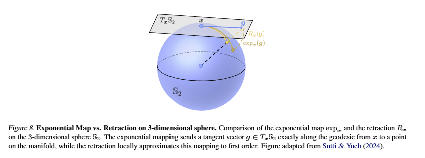
两个概念: 指数映射(Exponential Mapping)和retraction。
- 指数映射是指对正切平面的向量,想象成一个柔软的绳子,沿着geodesic方向掉在流形上,绳子的终点的那个点就是映射的结果。
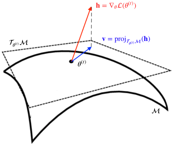
- 黎曼提出的在流形的正切空间内$T_{x}\mathcal M$,可以根据某一个向量$v \in T_{x}\mathcal M$做retraction 下图展示了在球体表面的两种方式,retraction可以看作是指数映射的一种一阶近似。
 回到刚才的问题:
SGD得到的是下图的红色向量,前面说的最大限度地在流形上找到更新步长和方向就变成了先在正确空间找到$h$的投影,再拿着投影去retraction找更新参数。
回到刚才的问题:
SGD得到的是下图的红色向量,前面说的最大限度地在流形上找到更新步长和方向就变成了先在正确空间找到$h$的投影,再拿着投影去retraction找更新参数。
 下面的公式就对应LERP&NORM那里的图。
Stochastic Gradient Descent on Riemannian Manifolds
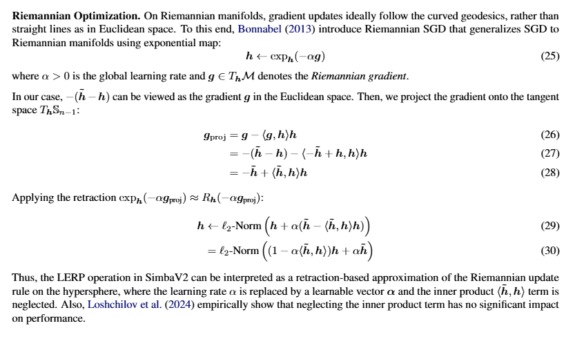
下面的公式就对应LERP&NORM那里的图。
Stochastic Gradient Descent on Riemannian Manifolds
 XQC: Well-conditioned Optimization Accelerates Deep Reinforcement Learning
| |
FlashSACDoubleCritic
num_qs默认为2,就是Double Critic。
| |
EnsembleCategoricalValue除了输出动作价值,还输出了动作价值的概率。 根据动作价值分布的方差和上下限范围,动态调整奖励的范围。
$$ \bar{r}_t = \frac{r _t}{\max \left(\sqrt{\sigma _{t,G}^2 + \epsilon}, G _{t,\max}/G _{\max}\right)} $$
| |
策略探索
- 最大熵动态调节:通过动作固定的标准差$\sigma_{tgt}$来计算目标熵$\mathcal H_{target}$,从而得到温度参数。
- 基于Zeta分布的噪声重复。
反向传播的梯度丢失问题
$\frac{\partial \mathcal L}{\partial a}$
Output Error - how much the final loss changes when the neuron’s output activation changes. This is the Upstream Gradient arriving from the output layer.
$\frac{\partial a}{\partial z}$ Activation Slope - the derivative of the activation function (e.g. ReLU or Sigmoid). This is the Local Gradient of this specific neuron.
$\frac{\partial z}{\partial w}$ Input Contribution - how much the raw neuron output changes when this specific weight changes. For a linear layer, this equals the input value x that originally activated this weight.
$\frac{\partial \mathcal L}{\partial w}$
Final Weight Gradient - the resulting Downstream Gradient handed to the optimizer. This single number tells the weight exactly how much and in which direction to change to reduce the loss.
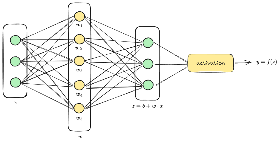
一般地,$a$是激活函数,$w$是网络参数,$\mathcal L$是loss, 是监督信号$y$和网络预测$y^{pre}$的函数:$\mathcal L(y, y^{pre})$,$z$是激活之前,网络的输出,对于单层网络,有:
$$ \frac{\partial\mathcal L}{\partial w}=\frac{\partial \mathcal L}{\partial a}\frac{\partial a}{\partial z}\frac{\partial z}{\partial w} $$ 两层网络: $$ \begin{aligned} \frac{\partial\mathcal L}{\partial w_{1}}&=\frac{\partial \mathcal L}{\partial a_{1}}\frac{\partial a_{1}}{\partial z_{1}}\frac{\partial z_{1}}{\partial w_{1}} \ &=\frac{\partial \mathcal L}{\partial a_{2}}\frac{\partial a_{2}}{\partial a_{1}}\frac{\partial a_{1}}{\partial z_{1}}\frac{\partial z_{1}}{\partial w_{1}} \ \end{aligned} $$
我们注意,当网络的层数继续增加,需要替换的是中间网络的前后级输出之间的梯度$\frac{a_{2}}{a_{1}}$,其他的梯度,都属于已知的,根据网络自身的结构就确定了。 $L$层网络:
$$ \begin{aligned} \frac{\partial\mathcal L}{\partial w_{1}}&=\frac{\partial \mathcal L}{\partial a_{1}}\frac{\partial a_{1}}{\partial z_{1}}\frac{\partial z_{1}}{\partial w_{1}} \ &=\frac{\partial \mathcal L}{\partial a_{L}}\frac{\partial a_{L}}{\partial a_{L-1}}\frac{\partial a_{L-1}}{\partial a_{L-2}}\cdots\frac{\partial a_{2}}{\partial a_{1}}\frac{\partial a_{1}}{\partial z_{1}}\frac{\partial z_{1}}{\partial w_{1}} \ \end{aligned} \tag{1} $$ 如果网络是$z=b+w\cdot x$的形式,$a_{l}=f_{l}(b_{l}+w_{l}\cdot a_{l-1})$,$z_{l}=b_{l}+w_{l}\cdot a_{l-1}$
$$ \frac{\partial a_{l}}{\partial a_{l-1}}=\frac{\partial a_{l}}{\partial z_{l}}\frac{\partial z_{l}}{\partial a_{l-1}}=\frac{\partial a_{l}}{\partial z_{l-1}}w_{l} $$
(1)变为:
$$ \begin{aligned} \frac{\partial\mathcal L}{\partial w_{1}}&=\frac{\partial \mathcal L}{\partial a_{1}}\frac{\partial a_{1}}{\partial z_{1}}\frac{\partial z_{1}}{\partial w_{1}} \ &=\frac{\partial \mathcal L}{\partial a_{L}}\frac{\partial a_{L}}{\partial z_{L-1}}w_{L}\frac{\partial a_{L-1}}{\partial z_{L-2}}w_{L-1}\cdots\frac{\partial a_{2}}{\partial z_{1}}w_{1}\frac{\partial a_{1}}{\partial z_{1}}\frac{\partial z_{1}}{\partial w_{1}} \ \end{aligned} \tag{2} $$
如果$\frac{\partial a_{l}}{\partial z_{l-1}}w_{l} < 1$,梯度更新传回到靠前的网络参数更新会被无限缩小。
ResNet
Rectified Linear Units (ReLU)是一种激活函数: 模拟了神经递质传递的过程,当信号强度大于0,就意味着通路打开,信号可以向后传递;当信号强度小于0,就意味着通路断开,该通路所代表的信息截断到此。 $$ \text{ReLU}(x) = x^+ = \max(0, x) = \frac{x + |x|}{2} = \begin{cases} x & \text{if } x > 0, \ 0 & \text{if } x \leq 0 \end{cases} $$
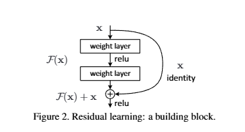
$\mathcal F(x)$学习到的是如果输入$x$,网络输出$\mathcal F(x)+x$和目标$y$之间的差距。假设我们刚开始训练网络,那么完全可以认为整个网络的输出就是输入,本身就建立了一个先验的对应关系;
$$ \frac{\partial a_{l}}{\partial a_{l-1}}=\frac{\partial a_{l}}{\partial z_{l}}\frac{\partial z_{l}}{\partial a_{l-1}}=\frac{\partial a_{l}}{\partial z_{l-1}}(w_{l} + 1) $$ 来看一下ResNet的反向传播:
$$ \begin{aligned} \frac{\partial\mathcal L}{\partial w_{1}}&=\frac{\partial \mathcal L}{\partial a_{1}}\frac{\partial a_{1}}{\partial z_{1}}\frac{\partial z_{1}}{\partial w_{1}} \ &=\frac{\partial \mathcal L}{\partial a_{L}}\frac{\partial a_{L}}{\partial z_{L-1}}(w_{l}+1)\frac{\partial a_{L-1}}{\partial z_{L-2}}(w_{l-1}+1)\cdots\frac{\partial a_{2}}{\partial z_{1}}(w_{1}+1)\frac{\partial a_{1}}{\partial z_{1}}\frac{\partial z_{1}}{\partial w_{1}} \ \end{aligned} \tag{2} $$
分析: 从正向理解:
- 避免遗忘:随着网络的深度增加,可以将前面的输入的信息,很好地保留到后面的网络中去
- 很多时候,其实输入$x$本身就很接近期望的输出了,需要变的那部分,放到网络里面去学习,就算学习的很差,也是基于原始输入做了不恰当的修改,不太影响原貌。
反向传播:
- 如上分析,避免因为网络参数接近于0导致的梯度回传失效
总结
HER和FlashSAC结合,可以解决机器人领域,尤其是灵巧手,人形机器人,动作空间维度大,成功率不高,数据昂贵等问题。是很好的预训练阶段的解决方案。