背景
在看《Bayesian models of cognition》时候,偶然看到了Importance Sampling的介绍,然后我就突然回忆起TRPO算法中,运用到了这个思路:
回忆:将理论上的新策略总收益迭代表达中,新策略($\tilde \pi$: policy being optimized)下的环境转移分布为权重的优势平均项,近似为行动策略($\pi$ : policy acting on env.)下的环境转移分布为权重的优势平均。
$$ L_\pi(\tilde \pi)=\eta(\pi) +\sum_{s\in \mathcal S}\rho_{\pi}(s)\sum_{a\in\mathcal A}\tilde \pi(a|s)A_\pi(s,a) $$
最大化$L_\pi(\tilde \pi)$其实就是最大化等式右边的第二项:$\sum_{s\in \mathcal S}\rho_{\pi}(s)\sum_{a\in\mathcal A}\tilde \pi(a|s)A_\pi(s,a)$
将该算法可工程化:基于数据的优化。利用行动策略$\pi$在环境中rollout数据,加上一个策略变化的KL限制,问题变为如下:
$$ \max _{\theta} \ L _{\theta _{\text{old}}}(\theta) \quad \text{s.t.} \quad \overline{D} _{\text{KL}}^{\rho _{\theta _{\text{old}}}}(\theta _{\text{old}}, \theta) \le \delta $$
观察第二个求和项: $$ \sum_{a\in\mathcal A}\tilde \pi(a|s)A_\pi(s,a) $$
其含义是待优化策略分布下,行动策略和环境交互过程中得到的优势的期望。但是在此时此刻,我们并不清楚待优化的策略分布是什么,跟当前的策略有什么变化,所以该部分无从求解。重要性采样(Importance Sampling)就是在这个时刻发挥了作用。我们无法预知整个$\pi$的分布,但是单点的计算是可以知道的$\pi(a_t|s_t)$:这一步可以叫做新策略下的老行动评估,实际的做法就是利用环境数据$s_t$产生高斯分布的期望和方差,构建一个分布,例如MultivariateNormal,然后基于这个分布计算行动$a_t$的单点概率。
$$ \sum _a \pi _\theta(a|s_n) A _{\theta _{\text{old}}}(s_n, a) = \mathbb{E} _{a \sim q} \left[ \frac{\pi _\theta(a|s_n)}{q(a|s_n)} A _{\theta _{\text{old}}}(s_n, a) \right] $$
Importance Sampling
该方法是为了解决已知一种分布$q(x)$,需要对另一种分布$p(x)$下的$f(x)$求期望的问题。
Changing the Sampling Problem: Assume that we want to evaluate an expectation of a function $f(x)$ with respect to a probability distribution $p(x)$ but have another distribution $q(x)$ that is easier to sample from. Further, assume that $q(x)> 0$ whenever $p(x)> 0$. We can introduce $q(x)$ into our expectation by multiplying and dividing by the same term, giving
$$ \begin{aligned} & \mathbb E_{p(x)}[f(x)] =\int f(x) p(x) dx=\frac{\int f(x) p(x) dx}{\int p(x) dx} \\ & =\frac{\int \frac{p(x)}{q(x)} f(x) q(x) dx}{\int \frac{p(x)}{q(x)} q(x) dx} \end{aligned} $$
Applying simple Monte Carlo to approximate these expectations, we obtain
$$ E _{p(\mathbf{x})}[f(\mathbf{x})] \approx \frac{ \frac{1}{m} \sum _{j=1}^{m} f(\mathbf{x}_j) \frac{p(\mathbf{x}_j)}{q(\mathbf{x}_j)} }{ \frac{1}{m} \sum _{j=1}^{m} \frac{p(\mathbf{x}_j)}{q(\mathbf{x}_j)} } $$
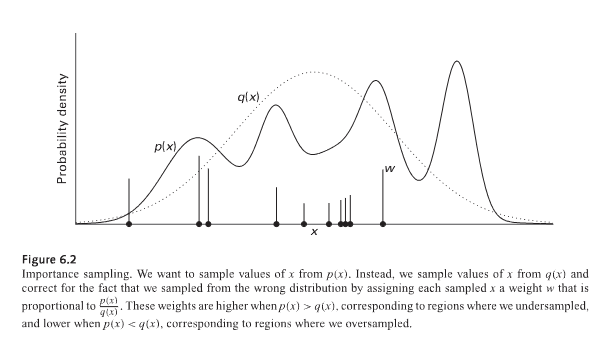
The ratios$\frac{p(x_{j})}{q(x_{j})}$ can be interpreted as “weights” on the sample $x_j$, correcting for the fact that they were drawn from $q(x)$ rather than $p(x)$ (see figure 6. 2 ). Samples that have higher probability under $p(x)$ than $q(x)$, and thus occur less often than they would if we were sampling from $p(x)$, receive greater weight. More formally, define the weight $w_j$ to be
$$ w_j = \frac{\frac{p(\mathbf{x}_j)}{q(\mathbf{x}_j)}}{\sum _{j=1}^m \frac{p(\mathbf{x}_j)}{q(\mathbf{x}_j)}} $$
$$ E_{p(\mathbf{x})}[f(\mathbf{x})] \approx \sum _{j=1}^{m} f(\mathbf{x}_j) w_j = \hat{\mu} _{IS}. $$
Analysis of Importance Sampling
It is instructive to compare the properties of the the importance sampling estimator $\hat{\mu} _{IS}$ with that of simple Monte Carlo. Under similar assumptions about $f(x)$ and $p(x)$ (with the significant addition that $q(x)> 0$ for all $x$ such that $p(x)> 0$), it is a consistent estimator of $\mu$, with $(\hat{\mu} _{IS}-\mu) \rightarrow 0$ almost surely as $m \rightarrow \infty$. It is also asymptotically normal, with
$$ \sqrt{m} (\hat{\mu} _{IS} - \mu) \to N(0, \sigma _{IS}^2) $$
in distribution, where $\sigma_{IS}^2 = E_{p(\mathbf{x})} \left[ \left( f(\mathbf{x}) - E_{p(\mathbf{x})}[f(\mathbf{x})] \right)^2 \tfrac{p(\mathbf{x})}{q(\mathbf{x})} \right]$. However, unlike simple Monte Carlo, $\hat{\mu}_{IS}$ is biased, with
$$ \begin{aligned} \hat{\mu} _{IS} - \mu = \frac{1}{m} \left( E _{p(\mathbf{x})} \left[ f(\mathbf{x}) \right] E _{p(\mathbf{x})} \left[ \tfrac{p(\mathbf{x})}{q(\mathbf{x})} \right] - E _{p(\mathbf{x})} \left[ f(\mathbf{x}) \tfrac{p(\mathbf{x})}{q(\mathbf{x})} \right] \right) \end{aligned} $$
which goes to zero as $m \rightarrow \infty$, but it can be substantial for smaller values of $m$. Despite being biased, there are several reasons why using an importance sampler can make sense even in cases where simple Monte Carlo can be applied. First, it allows a single set of samples to be used to evaluate expectations with respect to a range of distributions, through the use of different weights for each distribution. Second, the estimate produced by the importance sampler can have lower variance than the estimate produced by simple Monte Carlo. If the function $f(x)$ takes on its most extreme values in regions where $p(x)$ is small, the variance of the simple Monte Carlo estimate can be large. An importance sampler can have lower variance than simple Monte Carlo if $q(x)$ is chosen to be complementary to $f(x)$. In particular, the asymptotic variance of the sampler is minimized by specifying $q(x)$ as
$$ \begin{aligned} q(\mathbf{x}) \propto \left| f(\mathbf{x}) - \mathbb{E} _{p(\mathbf{x})} \left[ f(\mathbf{x}) \right] \right| p(\mathbf{x}) \end{aligned} $$
This is not a practical procedure since finding this distribution requires computing $\mathbb E_{p(x)} [ f(x)]$, but the fact that the minimum variance sampler need not be $p(x)$ illustrates that importance sampling can sometimes provide a lower variance estimate of an expectation than simple Monte Carlo.
小节
从重要性采样的分析来看,TRPO对策略更新的KL限制,恰巧迎合了$p(x)$和$q(x)$分布差异不要太大的要求,使得对期望的估计保持在较低的方差;且采样数量$m$的增大,可以很好地让估计逼近真实值,这也为我们设计或者使用rollout trajectory提供了理论支撑。