学习RL(六)

DDPG与TD3：连续动作空间的深度确定性策略梯度

Open AI Spinning Up - DDPG - DDPG（Deep Deterministic Policy Gradient） Deep Deterministic Policy Gradient (DDPG) is an algorithm which concurrently learns a Q-function and a policy. It uses off-policy data and the Bellman equation to learn the Q-function, and uses the Q-function to learn the policy.

本文记录我在学习DDPG（Deep Deterministic Policy Gradient）和TD3（Twin Delayed DDPG）的过程，梳理清楚他们产生的背景，核心思想，特点以及我在实现过程中遇到的问题记录和解决。

1. 背景与动机

DQN在离散动作空间表现出色。然而，在许多实际控制任务中（如机器人控制、自动驾驶等），动作空间是连续的。DQN无法计算所有的$Q(s,a)$,代价太大。随着动作空间维度的提升，离散化动作空间带来的成本增加呈指数级别。

DDPG正是为解决连续动作空间控制问题而设计的。

2. DDPG核心思想

参考Policy Gradient和PPO，DDPG和TD3想要通过梯度下降的方法对Policy做优化(调节$\theta$)，在训练结束的时候，具有一个最优化的$\theta$，使得$Q(s,a)$$\big(a=\mu_\theta(s)\big )$最大化，还要借鉴DQN当中使用到的replay buffer: $\mathcal D$和target network等技术，来提升训练的稳定性和效率。DQN通过Q网络¹和target_Q网络²分别近似$Q^\star(s,a)$和$Q^\star(s’,a’)$，

根据Bellman Optimality Equation:

$$ Q^\star(s,a) = \mathbb{E}[r(s,a) + \gamma \max_{a’} Q^\star(s’, a’)] $$

从target Q网络中获取最优action的代码：

1

self.Q_target_network(non_final_next_states).max(1).values

通过$\mathcal D$中的采样数据形成batch,计算上式中的TD目标$r + \gamma \max_{a’} Q^\star(s’, a’)$。

针对连续动作空间，DDPG相对于DQN改进的地方主要在于，DQN网络输入只有状态$s$，输出是每个离散动作对应的Q值，无法利用动作网络$\mu(s)$的输出直接计算Q值，那么，就改造$Q _{\phi}$网络的输入为状态和动作的组合$(s,a)$，输出对应的Q值，这样就可以直接利用$\mu(s)$的输出作为Q网络的输入，根据计算结果来优化$\mu(s)$的参数$\theta$，使得在状态$s$下输出的动作$a$能够最大化Q值。

为了找到$\max_{a’} Q^\star(s’, a’)$里面的$a’$,使用$\mu _{\theta _{target}}(s’)$得到，即target_actor。并且每隔一段时间就将critic和actor网络的参数复制到target_critc和target_actor网络中(或者是软更新)。

所以优化的目标就是: $Q^\star(s,a)\approx Q_{\phi} ^\star (s,\mu_\theta(s))$：被优化的参数是$\theta$和$\phi$。

下面是DDPG的核心优化流程：

• 网络$Q_\phi(s,a)$用于评价当前policy $\mu_{\theta}$的critic，网络$Q_{\phi_{targ}}(s,a)$用于给出目标价值，主要目的是提供稳定的训练目标参考¹。借助MSBE(mean-squared Bellman Error)更新Critic网络$Q_\phi$的参数$\phi$：

$$ \mathcal L(\phi,\mathcal D) = \mathbb E_{(s,a,r,s’)\sim \mathcal D} \bigg[ \bigg( r + \gamma(1-d) Q_{\phi_{targ}}(s’,\mu_{\theta_{targ}}(s’)) - Q_\phi(s,a) \bigg)^2 \bigg] $$

$d=1 \ if \ s’ \ is \ terminal \ else \ 0$，$\mathcal D$是经验回放缓冲区。

• actor网络$\mu_\theta(s)$的更新: $Q_{\phi}(s,a)$更新之后，Actor网络$\mu_\theta$优化的目标是：

$$ \max_{\theta} \mathbb{E}_{s \sim \mathcal{D}} [Q _{\phi}(s, \mu _{\theta}(s))] $$

• $\mu_\theta$更新之后，对环境重新交互，生成的$(s,a,r,s’)$加入回放缓冲区$\mathcal D$，重复上述过程。

代码实现

3 DDPG的特点

3.1 确定性策略

与PPO等随机策略不同，DDPG采用确定性策略（Deterministic Policy）：

$$ a = \mu_\theta(s) $$

这意味着给定状态时，Actor直接输出一个确定的动作，而不是动作的概率分布。

3.2 Actor-Critic架构

DDPG采用经典的Actor-Critic架构：

• Actor（策略网络）：$\mu_\theta(s)$ - 输入状态，输出确定性动作
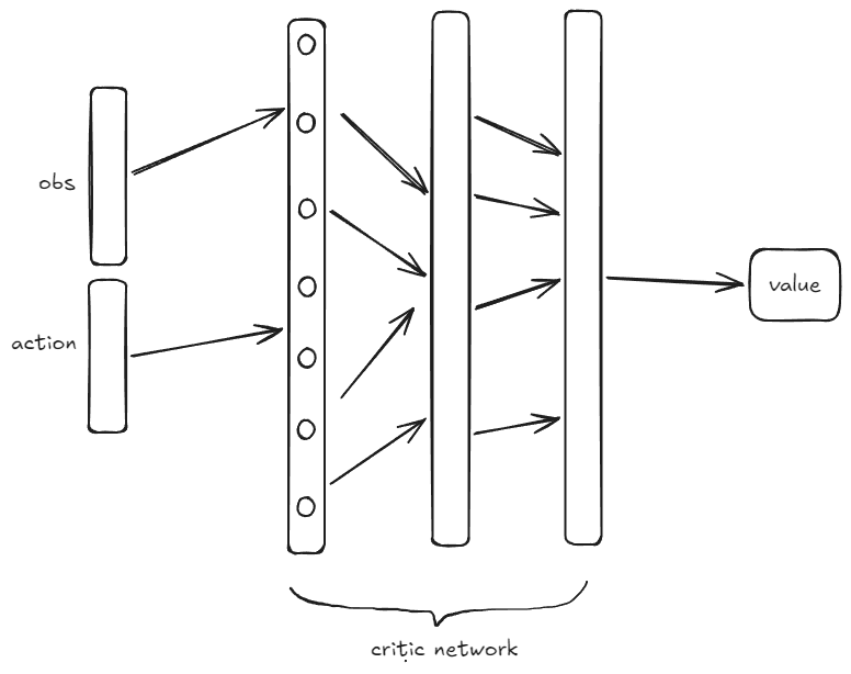
• Critic（价值网络）：$Q_\phi(s, a)$ - 输入状态和动作，输出Q值

Critic网络的输入是状态+动作的组合，这是与PPO的重要区别。

3.3 经验回放与目标网络

DDPG借鉴了DQN的两个关键技术：

1. 经验回放（Replay Buffer）：存储$(s_t, a_t, r_t, s_{t+1})$ tuples，训练时随机采样，打破时间相关性
2. 目标网络（Target Network）：使用延迟更新的目标网络计算TD目标，提高训练稳定性

经验回放的四大优势

使用replay buffer有以下几个关键优势：

1. 打破时序关联：一条轨迹中的$(s_t,a,r,s_{t+1})$具有强相关性，直接用于训练会导致网络难以收敛。随机采样打散了这种关联。

2. 提高数据效率：在奖励稀疏的环境中（如机器人抓取），智能体可能需要探索很长时间才能获得少量有价值的transition。经验回放可以重复利用历史数据，多次从中采样进行更新，显著降低了数据采集成本。

3. 支持优先采样：可以在不同训练阶段选择更有价值的transition进行学习。例如，当需要更多更新Actor时，可以优先选择那些更能提升策略的样本。

4. 容纳多样化经验：回放缓冲区可以存储来自不同策略产生的数据，使最终学到的策略能够适应多变的环境，增强泛化能力。

3.4 探索策略

由于采用确定性策略，为了保证数据的多样性，需要对$\mu_\theta(s)$添加探索噪声:

$$ a = \mu_\theta(s) + \mathcal{N} $$ 我在实现get_action函数时候，犯了错：网络的输出本质上是一个在[-1, 1]范围内的动作值（因为Actor网络最后一层使用了tanh激活函数），所以，需要先将噪声也映射到[-1, 1]范围内，再和归一化的动作相加，最后再将动作映射到环境的实际动作空间：

 1
 2
 3
 4
 5
 6
 7
 8
 9
10
11
12
13
14
15
16
17
18
19
20
21
22
23
24
25
26

def get_action(self, obs, noise_scale=None):
        """
            get action according to current policy self.actor and exploration noise,
            clip the result to valid one

            Parameters:
				state - one observation from env
							Shape: (dimension of observation,1)
                noise_scale - noise reduce scalar，None means use  self.action_noise, otherwise use 
                            noise_scale * self.action_noise

			Return:
				action_with_noise - output from actor_model is mean_action;
                clip (mean_action + noise) with the action_space_high and action_space_low to make sure output is in boundary
                                Type: tensor
        """

        # mean action
        mean = self.actor(obs)
        mean_action = mean.detach().numpy().flatten()
        noise_scale = noise_scale if noise_scale is not None else self.action_noise
        noise = np.random.normal(0, noise_scale, size=mean_action.shape)
        action_with_noise = mean_action + noise
        action_with_noise = np.clip(action_with_noise,-1, 1)
        action_with_noise = action_with_noise * (self.action_space_high - self.action_space_low) / 2 + (self.action_space_high + self.action_space_low) / 2
        return action_with_noise

4. DDPG算法流程

5. TD3：双延迟深度确定性策略梯度

TD3是DDPG的改进版本，针对DDPG的Q值过估计问题提出了三项关键改进。

5.1 三大改进

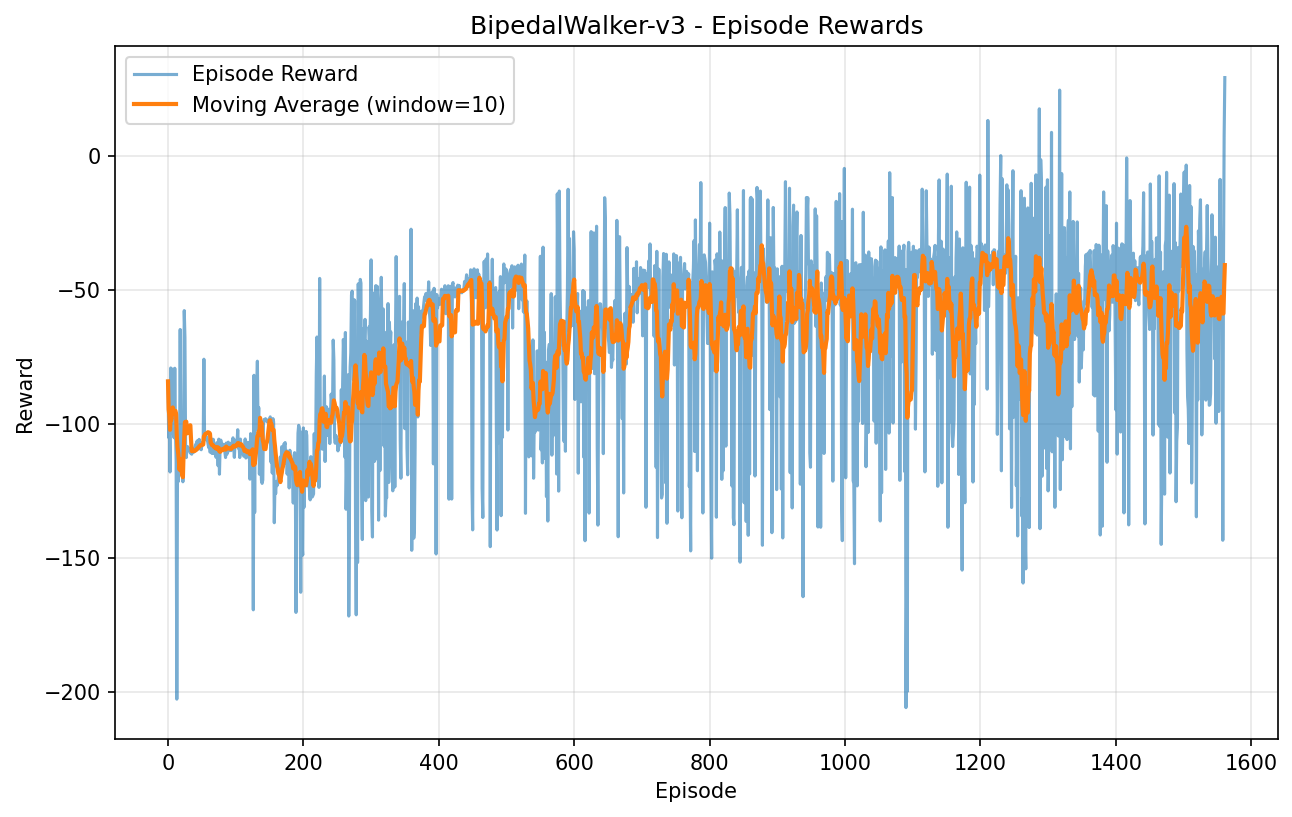
在使用DDPG训练过程中，遇到了Q值过估计的问题，导致训练不稳定，典型的现象就是reward先上升，然后下降，无法逼近预期的reward。TD3通过以下三项改进来解决这个问题：

1. 截断双Q学习（Clipped Double Q-Learning）

使用两个独立的Critic网络$Q_{\phi_1} ^{\text{target}}$和$Q_{\phi_2}^{\text{target}}$在代码中是class DoubleQCritic:

 1
 2
 3
 4
 5
 6
 7
 8
 9
10
11
12
13
14
15
16
17
18
19

class DoubleQCritic(nn.Module):
    def __init__(self, obs_size, action_size, output_size,net_width=128):
        super(DoubleQCritic, self).__init__()
        self.crtic1_layer1 = nn.Linear(obs_size + action_size, net_width)
        self.crtic1_layer2 = nn.Linear(net_width, net_width)
        self.critic1_output_layer = nn.Linear(net_width, output_size)

        self.crtic2_layer1 = nn.Linear(obs_size + action_size, net_width)
        self.crtic2_layer2 = nn.Linear(net_width, net_width)
        self.critic2_output_layer = nn.Linear(net_width, output_size)

    def forward(self, obs, action):
        sa = torch.cat([obs, action], 1)
        critic1_actv1 = F.relu(self.crtic1_layer1(sa))
        critic1_actv2 = F.relu(self.crtic1_layer2(critic1_actv1))

        criti2_actv1 = F.relu(self.crtic2_layer1(sa))
        criti2_actv2 = F.relu(self.crtic2_layer2(criti2_actv1))
        return self.critic1_output_layer(critic1_actv2), self.critic2_output_layer(criti2_actv2)

取较小的Q值作为目标：

$$ y = r + \gamma \min_{i=1,2} Q_{\phi_i}^{\text{target}}(s’, \mu_{\theta_{\text{target}}}(s’) + \epsilon) $$

2. 目标策略平滑（Target Policy Smoothing）

在目标动作上添加小的随机噪声，防止Actor过度拟合Q函数的尖峰：

$$ a’ = \mu_{\theta_{\text{target}}}(s’) + \text{clip}(\epsilon, -c, c) $$ 其中$\epsilon \sim \text{clip}(\mathcal{N}(0, \sigma), -c, c)$为target policy noise:

Trick Three: Target Policy Smoothing. TD3 adds noise to the target action, to make it harder for the policy to exploit Q-function errors by smoothing out Q along changes in action.

3. 延迟策略更新（Delayed Policy Updates）

Actor网络更新频率低于Critic网络（例如每2步更新一次Actor），避免策略在Critic未收敛时产生错误引导。

5.2 TD3算法伪代码

5. 实现细节与经验

TD3代码实现

5.1 关键实现要点

1. 动作范围映射：Actor网络输出通常在[-1, 1]，需要根据环境action_space映射到实际范围：

   1	action = action * (env.action_space.high - env.action_space.low) / 2 + (env.action_space.high + env.action_space.low) / 2

2. 目标网络软更新：

   1 2	for target_param, param in zip(target.parameters(), online.parameters()): target_param.data.copy_(tau * param.data + (1 - tau) * target_param.data)

   3. 训练前，replay buffer需要预热，收集一定数量的随机交互数据，确保训练初期有足够的样本。

   1 2 3 4 5 6 7 8 9 10 11 12 13 14 15 16 17 18 19 20 21 22 23 24 25 26 27

   for i_episode in count(): # each episode should env.reset() first observation, info = env.reset() state = torch.tensor(observation, dtype=torch.float32).unsqueeze(0) for t in count(): if currentStep > time_to_update: action = ddpg.get_action(state) else: action = env.action_space.sample() observation, reward, terminated, truncated, _ = env.step(action) currentStep += 1 episode_reward += reward done = terminated or truncated if terminated: next_state = None else: next_state = torch.tensor(observation, dtype=torch.float32).unsqueeze(0) reward_tensor = torch.tensor([reward]) action_tensor = torch.tensor(action, dtype=torch.float32).unsqueeze(0) ddpg.add_replay_memory(state, action_tensor, next_state, reward_tensor) state = next_state if currentStep > time_to_update: ddpg.train_model()

5.2 常见问题与调参经验

根据实际实现经验，DDPG/TD3常见问题：

1. Q值过估计：训练过程中Q值可能急剧上升，导致策略崩溃

   • 解决：使用TD3的双Q网络和目标策略平滑

2. 训练不稳定：rewards先变大后变小

   • 解决：使用较小的学习率，TD3的延迟更新策略

3. 探索不足：动作噪声衰减过快

   • 解决：保持恒定的探索噪声，或使用递减策略

5.3 超参数推荐

我的超参配置

6. PyTorch代码实现

6.1 Actor网络

Actor网络输入状态，输出一个确定性动作（使用tanh将输出限制在[-1, 1]）：

 1
 2
 3
 4
 5
 6
 7
 8
 9
10
11
12
13
14
15

import torch
import torch.nn as nn
import torch.nn.functional as F

class Actor(nn.Module):
    def __init__(self, input_size, output_size, net_width=128):
        super(Actor, self).__init__()
        self.layer1 = nn.Linear(input_size, net_width)
        self.layer2 = nn.Linear(net_width, net_width)
        self.output_layer = nn.Linear(net_width, output_size)

    def forward(self, obs):
        actv1 = F.relu(self.layer1(obs))
        actv2 = F.relu(self.layer2(actv1))
        return torch.tanh(self.output_layer(actv2))  # 输出范围 [-1, 1]

6.2 Q-Critic网络

Critic网络输入状态和动作的组合，输出Q值：

 1
 2
 3
 4
 5
 6
 7
 8
 9
10
11
12

class QCritic(nn.Module):
    def __init__(self, obs_size, action_size, output_size, net_width=128):
        super(QCritic, self).__init__()
        self.layer1 = nn.Linear(obs_size + action_size, net_width)
        self.layer2 = nn.Linear(net_width, net_width)
        self.output_layer = nn.Linear(net_width, output_size)

    def forward(self, obs, action):
        sa = torch.cat([obs, action], 1)  # 状态与动作拼接
        actv1 = F.relu(self.layer1(sa))
        actv2 = F.relu(self.layer2(actv1))
        return self.output_layer(actv2)

6.3 Double Q-Critic网络（TD3）

 1
 2
 3
 4
 5
 6
 7
 8
 9
10
11
12
13
14
15
16
17
18
19
20
21
22
23
24

class DoubleQCritic(nn.Module):
    """双Q Critic，用于TD3"""
    def __init__(self, obs_size, action_size, output_size, net_width=128):
        super(DoubleQCritic, self).__init__()
        # 第一个Q网络
        self.critic1_layer1 = nn.Linear(obs_size + action_size, net_width)
        self.critic1_layer2 = nn.Linear(net_width, net_width)
        self.critic1_output_layer = nn.Linear(net_width, output_size)
        # 第二个Q网络
        self.critic2_layer1 = nn.Linear(obs_size + action_size, net_width)
        self.critic2_layer2 = nn.Linear(net_width, net_width)
        self.critic2_output_layer = nn.Linear(net_width, output_size)

    def forward(self, obs, action):
        sa = torch.cat([obs, action], 1)
        # Q1
        c1_actv1 = F.relu(self.critic1_layer1(sa))
        c1_actv2 = F.relu(self.critic1_layer2(c1_actv1))
        q1 = self.critic1_output_layer(c1_actv2)
        # Q2
        c2_actv1 = F.relu(self.critic2_layer1(sa))
        c2_actv2 = F.relu(self.critic2_layer2(c2_actv1))
        q2 = self.critic2_output_layer(c2_actv2)
        return q1, q2

7. Stable-Baselines3使用示例

除了自己实现，Stable-Baselines3中提供了高质量的TD3和DDPG实现：

1
2
3
4
5
6
7
8
9

from stable_baselines3 import TD3, DDPG

# TD3
model = TD3("MlpPolicy", "HalfCheetah-v4", verbose=1)
model.learn(total_timesteps=10000)

# DDPG
model = DDPG("MlpPolicy", "Pendulum-v1", verbose=1)
model.learn(total_timesteps=10000)

继承关系：

1
2
3

OffPolicyAlgorithm
    └── TD3 (Twin Delayed DDPG)
        └── DDPG (Deep Deterministic Policy Gradient)

8. 总结

DDPG是将深度学习与确定性策略梯度结合的里程碑式算法，为连续动作空间控制提供了有效解决方案。TD3通过三项关键改进显著提高了训练稳定性和性能，是目前处理连续控制问题的默认选择之一。

参考资料

1. Human-level control through deep reinforcement learning (DQN) - Mnih et al., Nature, 2015
2. DDPG Paper - Lillicrap et al., 2015
3. TD3 Paper - Fujita et al., 2018
4. OpenAI Spinning Up - DDPG
5. OpenAI Spinning Up - TD3
6. Stable-Baselines3 Documentation